In this post I hope to unveil new possibilities on a comprehensive review of Mathematica 14. What with the data that I've been discussing in my prior Wolfram Community post on Mathematica 13, I should make a post about Mathematica 14. Now, the data (World Cities Database | Simplemaps.com https://simplemaps.com/data/world-cities) is about important city data. The thing about Mathematica 14 is that it allows us to convert data into a structured association, which is similar to a dictionary by importing from a CSV file and then converting numeric data from strings into numbers. We can then prepare the data for analysis and visualization by organizing it into meaningful attributes like city ID, name, population, geographic coordinates, elevation, and yes there is geographical visualization, of population data.
cityData =
  Import["/Users/deangladish/Downloads/simplemaps_worldcities_basicv1.\
77/worldcities.csv"];
processedData = AssociationThread[
     {"CityID", "CountryAbbreviation", "CityName",
      "PopulationThousands", "LatitudeDegrees", "LongitudeDegrees",
      "ElevationMeters"}, #] & /@
   cityData[[2 ;;, {1, 5, 2, 10, 3, 4, 7}]];
processedData =
  processedData /.
   s_String :> ToExpression[s] /; StringMatchQ[s, NumberString];
GeoGraphics[{
  Table[{
    ColorData["Rainbow"][Log10[city["PopulationThousands"]]],
    Tooltip[
     Disk[
      GeoPosition[{city["LatitudeDegrees"], city["LongitudeDegrees"]}],
      Quantity[0.1*Log10[city["PopulationThousands"]], "Kilometers"]
      ],
     city["CityName"]]},
   {city, processedData}]},
 GeoBackground -> "CountryBorders",
 ImageSize -> Large,
 GeoProjection -> "Mercator"]
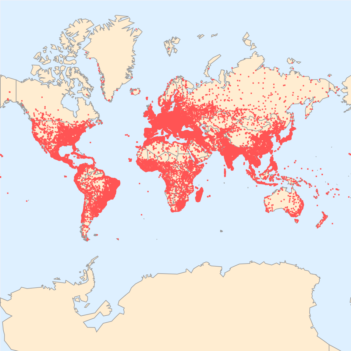
Typically when we make geographic maps that display cities we do it in plain English which means that we use English words and people have some idea of how we can stuff these maps in our brain to have some familiar language there. And that's sort of what Mathematica 14 is for, I thought this update wasn't going to come out for a long time; in a sense, the mathematical notation of the future is computational notation and that's what we spend much of our Mathematica installations trying to build is a consistence of computational notation, in most cases English having that as the backstop. Even if there might be some /@ notation, that's the thing that the experts do and now it's triple @ sign, in the end we have @ Apply and you kind of know what that means. In GeoGraphics we can display cities as colored disks whose color intensity and size depends..on their population. The colors being derived from a logarithmic scale, we can effectively manage wide ranges of population.
cityData =
  Import["/Users/deangladish/Downloads/simplemaps_worldcities_basicv1.\
77/worldcities.csv"];
processedData = AssociationThread[
     {"CityID", "CountryAbbreviation", "CityName",
      "PopulationThousands", "LatitudeDegrees", "LongitudeDegrees",
      "ElevationMeters"}, #] & /@
   cityData[[2 ;;, {1, 5, 2, 10, 3, 4, 7}]];
processedData =
  processedData /.
   s_String :>
    ToExpression[If[s == "", "0", s]] /;
     StringMatchQ[s, NumberString | ""];
points = Table[With[{
     popLog = Log[10,
       Max[city["PopulationThousands"], 1]
       ]
     },
    {
     RGBColor[ColorData["Rainbow"][1 - popLog/7]],
     PointSize[0.001 + 0.0001*popLog],
     Tooltip[
      Point[{city["LongitudeDegrees"], city["LatitudeDegrees"]}],
      city["CityName"]]
     }],
   {city, processedData}];
Graphics[points,
 Axes -> True, Frame -> True,
 AxesLabel -> {"Longitude (°)", "Latitude (°)"},
 PlotLabel -> "World Cities by Population",
 PlotRange -> {{-180, 180}, {-90, 90}},
 ImageSize -> Large,
 FrameLabel -> {None, None, "World Cities Visualization", None},
 Background -> Lighter[RGBColor[95/255, 4/255, 85/255], 0.9]]
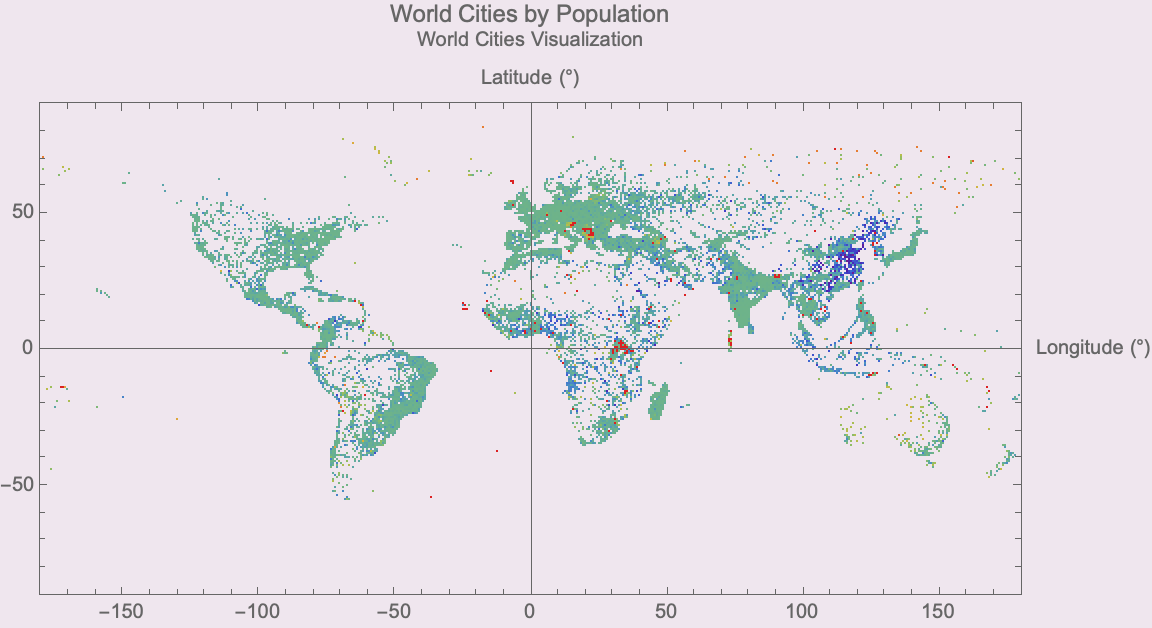
The map includes tooltips with city names and uses the projection Mercator, and that is how we get the context of geographical - we display the borders of the countries. What matters, and what doesn't? In Physics you can say I'm throwing an object off the Tower of Pisa or something and does it matter, the spikes or the edges? It's just the mass, air resistance in that case there wouldn't be a vacuum or so on. The thing we've learnt is that less matters than we might have thought. Because if we could handle missing data and include custom visualization via our Mathematica 14 segments which adapt the processed city data to replace missing population figures ("") with zeros, which gives us the stability that we need in logarithmic calculations..we can visualize the data in a scatter plot that is non-geographical. But it can also be geographical, it's not my personal preference to do that but we can, and we can use point size and color to represent population logs. And the graphical adjustments that we make, we highlight the distribution of the data..across global latitudes and longitudes, which offers a clear visual summary of worldwide urban centers.
rawData = {"0001,US,New York,8230,40.7128,-74.0060,10",
   "0002,GB,London,8982,51.5074,-0.1278,11",
   "0003,JP,Tokyo,13929,35.6895,139.6917,40",
   "0004,FR,Paris,2148,48.8566,2.3522,35",
   "0005,CA,Toronto,2731,43.6510,-79.3470,76",
   "0006,AU,Sydney,5312,33.8688,151.2093,58",
   "0007,BR,Rio de Janeiro,6748,22.9068,-43.1729,2",
   "0008,ZA,Cape Town,4337,33.9249,18.4241,42",
   "0009,IN,Mumbai,12478,19.0760,72.8777,14",
   "0010,CN,Shanghai,24150,31.2304,121.4737,4",
   "0011,EG,Cairo,9500,30.0444,31.2357,23",
   "0012,RU,Moscow,12500,55.7558,37.6173,156",
   "0013,DE,Berlin,3645,52.5200,13.4050,34",
   "0014,MX,Mexico City,8910,19.4326,-99.1332,2250",
   "0015,IT,Rome,2873,41.9028,12.4964,21",
   "0016,ES,Madrid,6642,40.4168,-3.7038,667",
   "0017,TR,Istanbul,15462,41.0082,28.9784,39",
   "0018,KR,Seoul,9776,37.5665,126.9780,38",
   "0019,AR,Buenos Aires,2890,34.6037,-58.3816,25",
   "0020,NG,Lagos,13900,6.5244,3.3792,11",
   "0021,US,Chicago,2715,41.8781,-87.6298,181",
   "0022,US,Los Angeles,3990,34.0522,-118.2437,89",
   "0023,CA,Vancouver,631,49.2827,-123.1207,70",
   "0024,BR,São Paulo,12300,23.5505,-46.6333,760",
   "0025,IN,Delhi,16700,28.7041,77.1025,216",
   "0026,JP,Osaka,8823,34.6937,135.5023,12",
   "0027,IT,Milan,3200,45.4642,9.1900,120",
   "0028,FR,Marseille,861,43.2965,5.3698,12",
   "0029,ES,Barcelona,5512,41.3851,2.1734,12",
   "0030,EG,Alexandria,5018,31.2156,29.9553,5"};
cityIdentifierCorrections = {888 -> 887, 3208 -> 3210, 5478 -> 5477,
   8559 -> 8558};
processedData = (
     <|"CityID" -> ToExpression[#[[1]]],
      "CountryAbbreviation" -> #[[2]],
      "CityName" -> #[[3]],
      "PopulationThousands" -> ToExpression[#[[4]]],
      "LatitudeDegrees" -> ToExpression[#[[5]]],
      "LongitudeDegrees" -> ToExpression[#[[6]]],
      "ElevationMeters" -> ToExpression[#[[7]]],
      "CityIdentifier" -> (ToExpression[#[[1]]] /.
         cityIdentifierCorrections)|>
     ) & /@ (StringSplit[#, ","] & /@ rawData);
Dataset[processedData]
minElevation = Min[processedData[[All, "ElevationMeters"]]];
maxElevation = Max[processedData[[All, "ElevationMeters"]]];
Graphics[{
  Table[
   {
    ColorData[
      "Rainbow"][(city["ElevationMeters"] -
        minElevation)/(maxElevation - minElevation)],
    Disk[{city["LongitudeDegrees"], city["LatitudeDegrees"]},
     0.01*Sqrt[city["PopulationThousands"]]],
    Black,
    Text[city["CityName"], {city["LongitudeDegrees"],
      city["LatitudeDegrees"]}, {0, -2}]
    },
   {city, processedData}
   ]
  }, Frame -> True, Axes -> True,
 AxesLabel -> {"Longitude (°)", "Latitude (°)"},
 PlotLabel -> "Visualization of City Elevations and Populations",
 ImageSize -> Large]
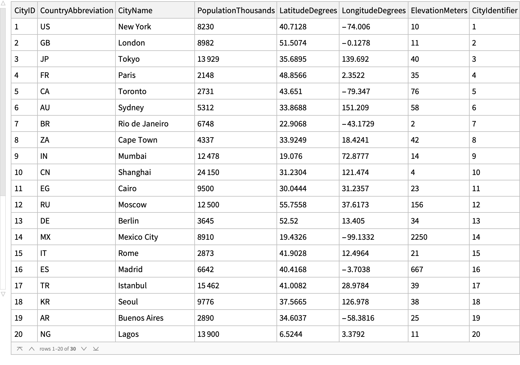
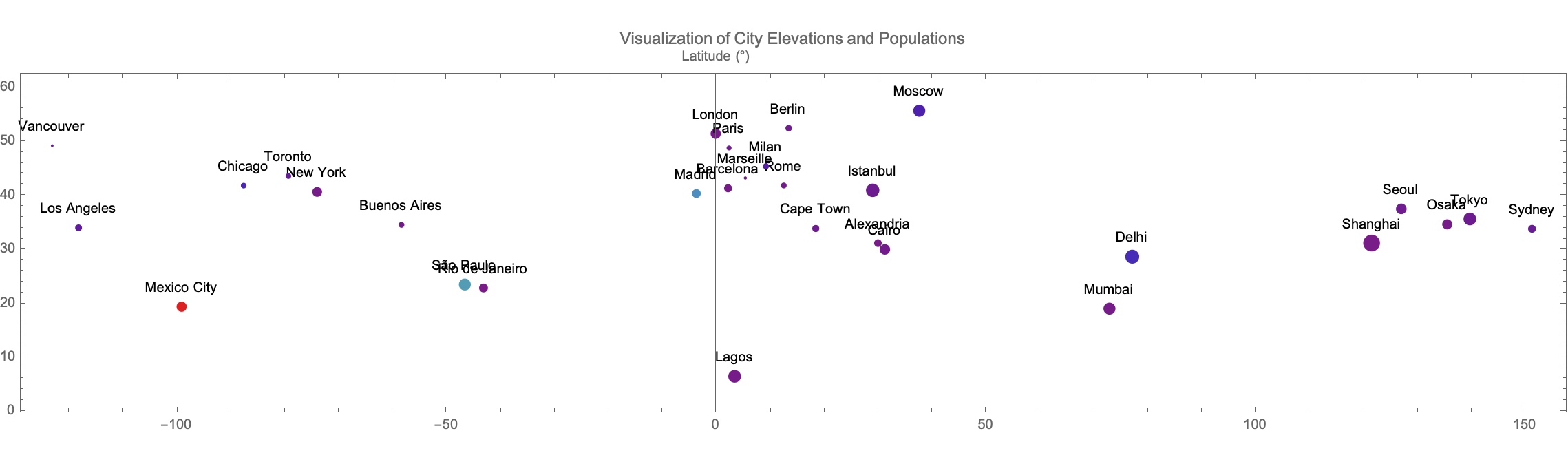
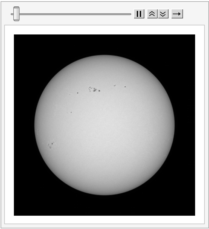
What about data processing for city attributes? If we could simulate or analyze the lifecycle of manually entered raw data for cities, correcting specific city identifiers using a predefined map of corrections, by basic optics experiments we could convert this data into structured forms suitable for a framework for designing and interpreting future analysis and visualization experiments, but Mathematica 14 simulates this process, broadening the application scope to include new computational fields like hyperelastic material modeling and electrostatic systems. Updates also extend to audio and video processing, reflecting Wolfram Language's adaptation to multimedia data handling. I've used Mathematica and it's full of interactive and informative content. Wolfram tools are designed with the best and brightest in talent which practically demonstrates how these technologies can be applied in real-world scenarios. For instance, if you were in Texas during the eclipse you would have thought it was the crack of dawn. But when we include interactive elements we can computationalize the progression of sunspot images over time and the creation of videos from these images which is particularly engaging, and that's why the only complex astronomical phenomenon is the astronomical phenomena that is understandable and accessible, accessibility is the utilization, of the combination of live solar images and historical data to draw comparisons between the current solar activity and significant events historically, like the stories of comparisons drawn between that and the Carrington Event of 1859. And with Mathematica 14 we can actually steer our exploration of the Ruliad. And I used to use Mathematica's earlier versions but now I can't, I've paid much more attention to the things of the past than the things of the current. But now we can finally answer those questions of how easy is it to compute a particular quantum function, what functions are hard to compute..if we follow that path well enough it would give us information about things we humans find easy, things we humans do not find easy, and it's a reasonable question. What functions are easy to compute for neural nets, what are not?
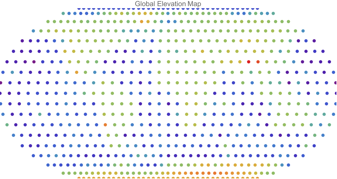
latitudeRange = Range[-90, 90, 10];
longitudeRange = Range[-180, 180, 10];
points =
  Flatten[Table[
    GeoPosition[{lat, lon}], {lat, latitudeRange}, {lon,
     longitudeRange}], 1];
elevations = GeoElevationData /@ points;
minElev = Min[elevations];
maxElev = Max[elevations];
normalizedElevations = Rescale[elevations, {minElev, maxElev}];
colors = ColorData["Rainbow"] /@ normalizedElevations;
pointColorPairs = Thread[points -> colors];
GeoGraphics[{PointSize[0.01], {#[[2]], Point[#[[1]]]} & /@
   Thread[{points, colors}]}, GeoProjection -> "Robinson",
 PlotLabel -> "Global Elevation Map", ImageSize -> Large,
 GeoBackground -> None]
And these solar images showcase Mathematica's robust capabilities in data manipulation, visualization, and geographical mapping, reflecting on the Mathematica 14 and what we did..let's take all those point weights and let's increase the values. Multiply them by 1.1, 1.2 whatever. The neural net keeps on getting adjusted and you do it differently, inflate the neural net weights. And what you see is the sun looks pretty good, look up in the writing that I did about this you know the 1.01 is looking pretty sun-like, by 1.05 the sun is starting to have bizarre solar flares sticking out of its head and so on, and by 1.07 the sun is kind of exploding there isn't a sun to be seen anymore. Given that exploded amped up network could one take that network and continue training it? My guess is yes. That training will just "revert" to what it learned before if it's the same training data. If it's a question of fine tuning I don't know the answer to that question. Generating diagrams that represent the evolution of these states and highlighting the increase in complexity and symmetry as the interaction progresses, after the completion phase, means that entanglement enters a propagation phase where the entangled states maintain their connection over distances.
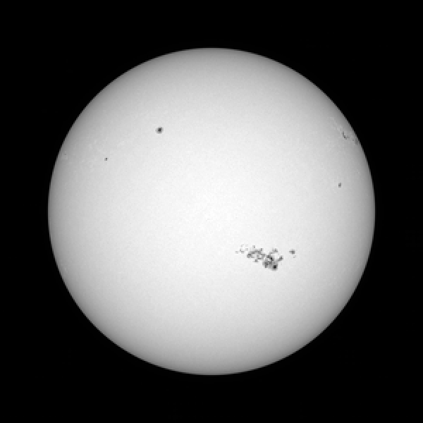
currentSolarImage =
 ResourceFunction["SolarImage"][
  DateObject[{2024, 5, 9, 0, 0, 0}, TimeZone -> 0],
  "ImageSize" -> 1200]

It can only do the things it was reflexively programmed to do or you could sign up for the future of computation, computational irreducibility. You're not going to be able to predict what will happen, when the expansion of the entangled network, as indicated by the simulation's generation of diagrams with increasing loops, representing the sustained entanglement. And that's why the sustained entanglement, lifecycle concludes in a phase where the entanglement either collapses, leading to a disentanglement of the quantum states, or transfers, where the entanglement is shifted onto other particles or states. And now we can actually visualize this entanglement via the graphics, geometry, and high-dimensional visualization of Mathematica 14.0 which introduces high-fidelity geometric regions, improving compatibility with CAD systems and enhancing graphical representation capabilities. What if you had some Computer Algebra System and you wanted to offer new tools for high-dimensional data visualization, aiding in more effective analysis and presentation of complex datasets? And that's why the Mathematica IDE has this tiny little support feature that guides us to the external services and improved import/export capabilities, so that we can integrate external services and boost the efficiency of importing and exporting data in various formats, facilitating better workflow integration and data management. Who knew that we could do all that because the world as we have built it, is built for us humans. Now, the natural world wasn't built for us humans although biological evolution has made us adapt to those niches, once we start colonizing Mars we're out of what we ever evolved to be in so to speak. Even the dynamic and reversible nature of quantum entanglement challenges the traditional notion of a wave function collapse as a singular, irreversible event. They're going to be able to walk up the steps, they're going to be able to open the door. So when you see the Wigner's Friends experiment, just simulated rolling around we can automate that, we can speed that up. And yes, it can have its own mop and the house was built so that it was freezing cold, shivering when the person who will be your Uber driver for the carriage or something like this, except I don't think this whole infrastructure for feeding the horses, using airships it's going to take a long time to go across the Atlantic, politically.
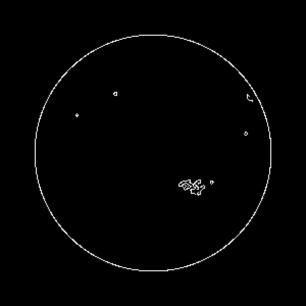
processedImage = ImageAdjust[currentSolarImage]
edgesImage = EdgeDetect[processedImage]
And in the Ruliad, if you hadn't had geometry and deduction as sort of a backdrop to some of the things that we were talking about within the arc of philosophical development and the continued discussion, and I will not continue..unless you never wanted to see the most active sunspot group again, of this solar cycle as it relates we would have had different things to talk about. Like how we can use Wolfram tools to practically demonstrate how these image composite and color replacement functions provide a commendable dive into the solar physics and now, we've got to process the parallels that we have processed, we've got to illustrate the capabilities of Mathematica-related phenomena whether it's encapsulating our awareness of space weather within a stellar 3d box like the AstroGraphics library, or just exploring the trajectory of current sunspot activity against historical events. But then there were dishwashers that are an excellent use case for supervised learning. Let's say you're going to have to grow your own food, and you apply that to us humans; there's always stuff to do that hasn't been automated. Remember that time, when we could choose, to say enough is enough, we could just hang out and sit back and have the machine peel the grapes and we'll just eat them and we'll just hang out don't do much else, hang out for our lives eating peeled grapes and that's all we'll do. It's the amazing gemstone. It's just a choice of somebody like me, I'm going to try to do that thing and as a species, as a society we could say enough is enough, we're done. When I saw the exploration of machine learning and neural networks, through these machine learning enhancements that we have got such as better support for neural network operations..I got so excited my face turned purple when I saw the natural language processing tools like TextSummarize, potentially impacting our statistical modeling via a more robust framework for machine learning with updated functions like Classify and Predict.
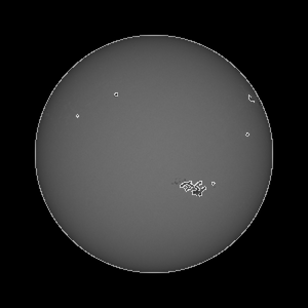
overlayImage = ImageCompose[currentSolarImage, {edgesImage, 0.5}]
dateRange =
 DateRange[DateObject[{2024, 5, 3, 0, 0, 0}, TimeZone -> 0], Now,
  "Day"]
And then there was later a thing that was a laptop size, that you could really just put in a bag and take with you. There are always pockets of quantum irreducibility places where we can have ideas, technology new ideas, there's a piece here there's a piece there. It's sort of inevitable we can put any number of patches on the more patches we put enough patches on the thing that's doing the patching is itself going to get very bloated. By the time we've got enough sort of axioms of our mathematical theory that everything's an axiom, you know the Riemann hypothesis or something like that, just that as an axiom. Eventually, it becomes very incoherent! Rolling around in those pockets of reducibility, those devices that sort of manage to do a little bit of jumping through computational reducibility; pick which device you could use. We never really get to transcend computational irreducibility..Pick another universe you can, but you'll never be able to communicate with our universe. So we're stuck, we the entities embedded in our universe. And the universe is just like us, and we are a part of the universe. It's inevitable by a diagonal argument that there will be computational irreducibility for us.
timeSeriesImages =
 ResourceFunction["SolarImage"][dateRange, "ImageSize" -> 1200]

Export["solar_evolution_slideshow.gif", ListAnimate[timeSeriesImages]];
spaceWeatherData =
  ResourceFunction[
    "SpaceWeatherData"][{DateObject[{2024, 5, 3, 0, 0, 0},
     TimeZone -> 0], Now}, {"ShortSolarXRayFlux",
    "LongSolarXRayFlux"}];
Something that's been a mistake of science for the last few hundred years, one has to realize that we have all a set of certain things that we're comfortable with. That's why when you see our fundamental understanding of the universe you've got to run very quickly with our new interfaces. Can you make that user interface remind people enough of something they knew, build that and give it to me. Give me the future experiments that could unveil new aspects of quantum reality, the quantum reality that provides your path forward for the experimental verification of the simulated outcomes. It can be pretty cartoonish, it's only the essentials that you need to capture. But it's really the case, when you're buzzing around and you're cryonically frozen, let's say I have a hamster. Perhaps it's very interesting, perhaps very disoriented. The things that are incredibly important to us today might not be the things that are incredibly important to us in the future, and that's another future of the Arrival of the Future! I just don't get why all of these kids worry about how many likes they get on Instagram. Every generation is always saying about the next one, I don't get why these people are communicating in emojis so you'd better pick up that phone! It's the kids you've really got to watch out for, they have all those cats and dogs and it's going to take a lot to slow the Earth down. The energy capacity to model sophisticated quantum scenarios, it's an interesting question how it compares with an interesting question, the energy, the ultimately deep thermal energy I don't know the answer that. I knew that calculation easily. If I'm typing in Wolfram Alpha, I can get to that calculation in a couple of minutes. I want to do a nuanced survey of the dynamics of quantum states and their interactions.
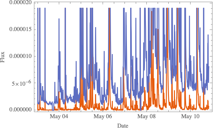
DateListPlot[spaceWeatherData, Joined -> True,
 PlotLegends -> {"Short Solar X-Ray Flux", "Long Solar X-Ray Flux"},
 FrameLabel -> {"Date", "Flux"}, PlotTheme -> "Scientific"]
Back these trends go cyclically on computers, in the cloud not only pushes the boundaries of our current understanding of quantum mechanics but also suggests a framework for designing and interpreting future quantum entanglement experiments. I will just press a button no clutter, everything's neatly folded stored in the cloud by a drone somewhere. It might actually be in the cloud there might be some giant platform, warehouse in the sky; whenever you need something it's just like let me get that thing, the library of stuff so to speak and that's the kind of thing one could imagine, if energy was cheap enough. But when it comes to computing right now, there's a certain energy cost in computing that doesn't need to be there.
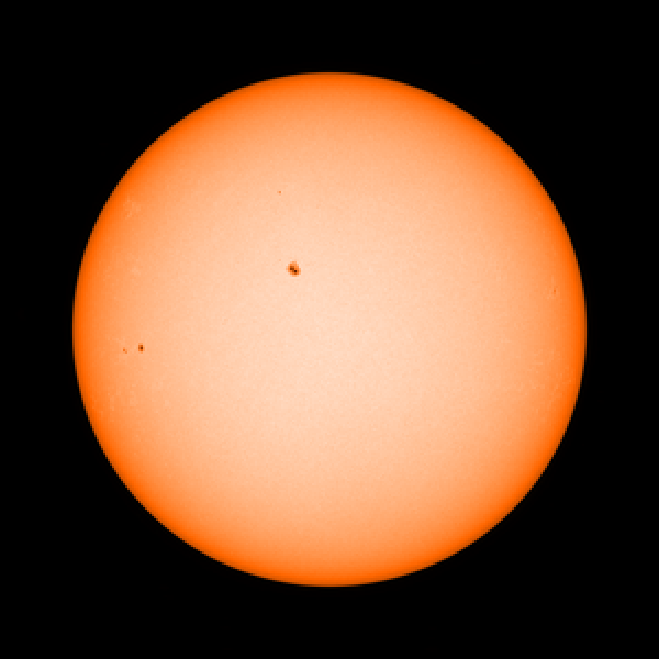
ResourceFunction["SolarImage"][
 DateObject[{2024, 4, 8, 13, 0, 0}, TimeZone -> 0],
 "ImageSize" -> 1200, "Colorize" -> True]
We know in principle how to do computing in a certain way and the maintenance and possibly the expansion of the entangled network, is indicated, by the simulation's generation of diagrams with increasing loops, representing the sustained entanglement. My life is officially ruined. I have been skipping the traditional notion of a wave function and the specific phases of entanglement and providing a visual and quantitative measure of the evolution of experiments that can measure the physical correlates of quantum diagrams, the crunchy, creamy, you know different kinds of food textures in your mouth they are literally correlated with the shapes of the proteins in foods.
convertedUnits = UnitConvert[Quantity[100, "Meters"], "Feet"]
currencyConversion =
 CurrencyConvert[Quantity[100, "USDollars"], "Euros",
  DateObject[{2023, 10, 1}]]
matrix = {{x, 1}, {1, x^2 + x + 1}};
finiteFieldMatrix = Map[ToFiniteField[#, 3] &, matrix, {2}]
inverseFFMatrix = Inverse[finiteFieldMatrix]
bspline = BSplineCurve[{{0, 0}, {1, 1}, {2, 0}, {3, 1}}];
RegionQ[bspline]
Comap[{Sin, Cos, Tan}, Pi/4]
ComapApply[{Plus, Times}, {{1, 2}, {3, 4}}]
FromRomanNumeral["MCMXCIV"]
RomanNumeral[1994]
model = Classify[{{1, 2} -> "A", {2, 3} -> "B", {3, 4} -> "C"},
   Method -> "NeuralNetwork"];
model[{2, 2}]
g = LayeredGraph[{1 <-> 2, 2 <-> 3, 3 <-> 1, 4 <-> 2, 5 <-> 3}];
HighlightGraph[g, PathGraph[{1, 2, 3}]]
CountDistinct[{1, 1, 2, 3, 2, 3, 3, 4}, (Mod[#1, 2] == Mod[#2, 2] &)]
UnitConvert[Quantity[10, "Miles"], "Kilometers"]
NSolve[x^5 - x + 1 == 0, x, Method -> "Monodromy"]
HermitianMatrixQ[HermitianMatrix[{{2, I}, {-I, 2}}]]
expr = {1, 2, 3, 4};
funcs = {#^2 &, Sqrt, Sin};
Comap[funcs, expr]
DigitSum[12345]
roman = RomanNumeral[2023]
integer = FromRomanNumeral[roman]
funcs = {Sin, Cos, Tan};
expr = Pi/4;
results = Comap[funcs, expr]
poly = x^3 + 2*x + 1;
ffPoly = ToFiniteField[poly, 5]
image = ExampleData[{"TestImage", "Lena"}]
image = Import["ExampleData/lena.tif"]
text = "The quick brown fox jumps over the lazy dog repeatedly.";
summary = TextSummarize[text]
So that means if you're eating fibers in muscle cells you have those active filaments that are in there, versus that you're having some quite different kind of protein from something else. Taste is all about the chemical interaction between the shapes of the molecules and how they bind to the taste receptors and the physicality of how the pieces are put together, how they smoosh on your tongue or whatever else. And trying to understand from the experimental "verification" of quantum entanglement, that's something that I think is somewhat in its infancy. For sound, we can create, yeah, a pretty much any sound we want it's still not easy you know if you say, make me a new kind of musical instrument. We're, starting to be able to do that and actually I think make me something that tastes like this. The implications of this research are far-reaching, potentially impacting information theory and our fundamental understanding of the universe.
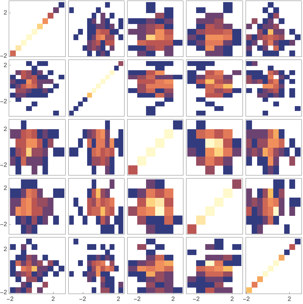
data = RandomVariate[NormalDistribution[], {100, 5}];
PairwiseDensityHistogram[data]
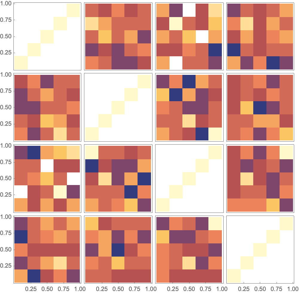
data = RandomReal[{0, 1}, {100, 4}];
PairwiseDensityHistogram[data]
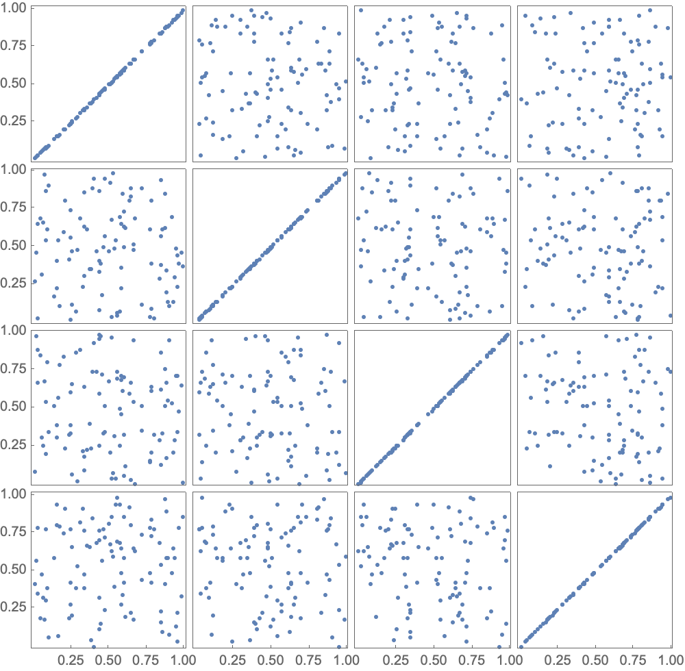
data = RandomReal[{0, 1}, {100, 4}];
PairwiseListPlot[data]
But it's not just the core language enhancements or the advances in mathematical computation, neither that nor the finite fields and equation solving, it's also that the release of Mathematica 14.0 brings us the variety of structured matrix types and operations, 14.0 has got our number on these decomposition techniques and enhanced support for interval matrices, boosting performance in linear algebra computations.
Therefore what Mathematica 14 does is it provides us with this ambient way of talking about the world as a sort of backdrop for the philosophy that we do, and we do contextualize the significance of events like eclipses in the context of universal computation. When talking about things like necessary truths, truths that don't rely on some coincidental fact about the universe..we see these things, in Mathematica 14.0 and its presentation of expansion across various domains in computational capabilities, demonstrating Wolfram Language's ongoing commitment to enhancing usability and integration with modern computational environments. But how can that be, when I see his longevity and the influence of his work, in his big, beautiful, basic new functions like Comap and ComapApply for applying lists of functions to expressions, and the subsequent errors that are introduced through copies over time...there are some basic systematic errors. It's almost like..the systematic errors that exist in several core functions that we use to increase their flexibility and performance via Mathematica 14, which handles these arguments and traceability in execution which has been refined and makes vector calculus, complex analysis, and integral transforms more palatable to users like us, and which sparks new functions for numerical integration in complex fields and not noting solutions for differential equations. If you asked me what I wrote in the past I wouldn't know but now, without proper attribution it's almost impossible to support advanced mathematical modeling. And so we present the visualizations of Mathematica 14, which expands its tools for working with finite fields and solving equations over these fields. Updated visualizations comparing efficient computation with the modern calculations of Mathematica 14 give us some new features like limiting the number of computed roots.


