


Integrate 
Integrate[f,x]
gives the indefinite integral  .
.
Integrate[f,{x,xmin,xmax}]
gives the definite integral  .
.
Integrate[f,{x,xmin,xmax},{y,ymin,ymax},…]
gives the multiple integral  .
.
Integrate[f,{x,y,…}∈reg]
integrates over the geometric region reg.
Details and Options
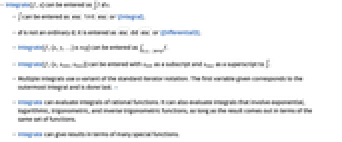

- Integrate[f,x] can be entered as ∫fx.
- ∫ can be entered as
 int
int or \[Integral].
 - is not an ordinary d; it is entered as
 dd
dd or \[DifferentialD].
 - Integrate[f,{x,y,…}∈reg] can be entered as ∫{x,y,…}∈regf.
- Integrate[f,{x,xmin,xmax}] can be entered with xmin as a subscript and xmax as a superscript to ∫.
- Multiple integrals use a variant of the standard iterator notation. The first variable given corresponds to the outermost integral and is done last. »
- Integrate can evaluate integrals of rational functions. It can also evaluate integrals that involve exponential, logarithmic, trigonometric, and inverse trigonometric functions, so long as the result comes out in terms of the same set of functions.
- Integrate can give results in terms of many special functions.
- Integrate carries out some simplifications on integrals it cannot explicitly do.
- You can get a numerical result by applying N to a definite integral. »
- You can assign values to patterns involving Integrate to give results for new classes of integrals.
- The integration variable can be a construct such as x[i] or any expression whose head is not a mathematical function.
- For indefinite integrals, Integrate tries to find results that are correct for almost all values of parameters.
- For definite integrals, the following options can be given:
-
Assumptions $Assumptionsassumptions to make about parameters GenerateConditions Automaticwhether to generate answers that involve conditions on parameters GeneratedParameters Nonehow to name generated parameters PrincipalValue Falsewhether to find Cauchy principal values - Integrate can evaluate essentially all indefinite integrals and most definite integrals listed in standard books of tables.
- In StandardForm, Integrate[f,x] is output as ∫fx.
Examples
open allclose allBasic Examples (4)
Visualize the area given by this integral:
Use  int
int to enter ∫ and
  dd
dd to enter :
Use  to enter the lower limit, then
  for the upper limit:
Scope (77)
Basic Uses (13)
Compute an indefinite integral:
Verify the answer by differentiation:
Use  intt
intt to enter a template
  and
and  to move between fields:
Include the constant of integration in an indefinite integral:
Compute a definite integral over a finite interval:
Use  dintt
dintt to enter a template
  and
and  to move between fields:
Integrate a function with a symbolic parameter:
An integral that only converges for some values of parameters:
Specify alternate assumptions to use:
Multiple integral with x integration last:
In StandardForm, the differential y precedes x:
Visualize the function over the domain of integration:
Integrals over standard regions:
The character ∈ can be entered as  el
el or ∈:
or ∈:
Enter a region specification  in an underscript using
  :
:
Use  rintt
rintt to enter a template
  and
and  to move between fields:
Integrals of vector- and array-valued functions:
Invoke NIntegrate automatically if symbolic integration fails:
Indefinite Integrals (10)
Generate an answer with a constant of integration:
Integrals of trigonometric functions:
Verify the previous answer via differentiation:
Create a nicely formatted table of integrals:
Rational functions can always be integrated in closed form:
Sometimes they involve sums of Root objects:
Integrals of general elementary functions:
Integrate returns antiderivatives valid in the complex plane where applicable:
A common antiderivative found in integral tables for  is
is ![log(TemplateBox[{{sec, (, x, )}}, RealAbs])](https://reference.wolfram.com/language/ref/Files/Integrate.en/75.png "log(TemplateBox[{{sec, (, x, )}}, RealAbs])") :
:
This is a valid antiderivative for real values of  :
:
On the real line, the two integrals have the same real part:
But the imaginary parts differ by  on any interval where
  is negative:
Similar integrals can lead to functions of different kinds:
Many integrals can be done only in terms of special functions such as Erf:
Generalizations of Log such as PolyLog and LogIntegral:
Hypergeometric functions such as Hypergeometric2F1:
Create a nicely-formatted table of special function integrals:
The variable of integration need not be a single symbol:
Definite Integrals (13)
Integrate a symbolic polynomial:
Integrate over a symbolic range:
Exponential and logarithmic functions:
Hyperbolic trigonometric functions:
Integrate a function with a vertical asymptote:
This can be viewed as a limit of the result of integration on a smaller interval:
Compute the integral of a function with two vertical asymptotes:
This can be viewed as a multivariate limit of the result of integration on a smaller interval:
Integrals over infinite intervals can be viewed as limits of integrals over finite domains:
The preceding is the limit as  of the integral from
  to
to  :
:
It is the bivariate limit of a finite integral:
When there are parameters, conditions that ensure convergence may be reported:
Integrals of elementary functions may produce special function answers:
Create a formatted table of definite integrals over the positive reals of special functions:
Integral along a complex line:
Along a piecewise linear contour in the complex plane:
Along a circular contour in the complex plane:
Plot the function and paths of integration:
Integrals of Piecewise and Generalized Functions (12)
Compute the indefinite integral of a Piecewise function:
In this case, the derivative of the integral equals the original function:
Integrate a discontinuous Piecewise function:
Except at the point of discontinuity, the derivative of g equals f:
Visualize the function and its antiderivative:
Integrate functions that are piecewise-defined:
Integrate a piecewise function with infinitely many cases:
Everywhere the derivative is defined, the derivative of maxInt equals the original function:
However, maxInt itself is discontinuous:
Compute a definite integral of a Piecewise function:
Compute the integral with a variable endpoint:
Visualize the function and its integral:
Compute definite integrals of piecewise functions such as Floor:
A composition of piecewise functions:
Compute the definite integral with a variable upper limit:
A function with an infinite number of cases:
Integrate over a finite number of cases using Assumptions:
The integral is a continuous function of the upper limit over the domain of integration:
Integrate generalized functions:
Indefinite integrals of generalized functions return generalized functions:
Integrate generalized functions over subsets of the reals:
Integrate an interpolating function:
Test that g is a correct antiderivative at x==3.5:
Nested Integrals (11)
Compute a second antiderivative of a function:
Compute the third antiderivative:
Integrate a function with respect to two different variables:
The mixed partial derivative gives the original function:
Generate a constant of integration for a single integral:
Generate constants for a nested integral with respect to the same variable:
This is the most general second antiderivative of the integrand:
Generate two functions of integration for a nested integral with respect to two variables:
This is the most general mixed antiderivative of the integrand:
Integrate over the rectangle from  to
to  :
:
Integrate in the opposite order:
Combine indefinite and definite integration:
Compute a rational double integral over a rectangular region:
This gives the volume of the shaded region:
Compute a trigonometric double integral over a rectangular region:
There is as much positive volume (dark gray) as negative (light blue):
Compute a polynomial double integral over the area between two curves:
Visualize the domain of integration and the volume corresponding to the integral:
Compute a triple integral over a rectangular prism:
Visualize the region of integration:
Integrate a multivariate function over a five-dimensional cube:
Integrate  over the unit ball in 4 dimensions:
Look up the coordinate ranges for hyperspherical coordinates in CoordinateChartData:
Also look up the volume factor:
Region Integrals (11)
Integrate a constant over a unit disk:
Enter the integral in typeset form:
Equivalently, integrate over a rectangular region and restrict to a disk using Boole:
The same integral expressed using Boole:
The same integral reduced to an iterated integral with bounds depending on the previous variables:
Plot the integrand over the integration region:
Express a normal definite integral using region notation:
Compare with the list notation:
With symbolic endpoints, assumptions are generated so that the region is non-degenerate:
Integrate over the unit circle:
Express the same integral as a one-dimensional integral using polar coordinates:
Integrate over a sphere of radius  :
:
Integrate over a finite set of points:
Regions can be given as logical combinations of inequalities:
Define the region as an ImplicitRegion and integrate directly over the region:
Visualize the domain of integration:
Integral over a three-dimensional region defined by inequalities:
Visualize 3D regions using RegionPlot3D:
Visualize the domain of integration:
Integrate a function with parameters, getting a piecewise result:
A region with infinitely many components:
Symbolic Features of Integrals (7)
Integrals involving unknown functions are done when possible:
Differentiate with respect to an endpoint, yielding the fundamental theorem of calculus:
Symbolic integrals can be differentiated with respect to parameters:
Differentiate with respect to a parameter that appears in both integrand and endpoints:
Use the Inactive form of Integrate:
Illustrate indefinite integral identities:
Verify the identities starting from the inactive forms:
Illustrate the basic commutation trick for differentiating under the integral sign:
Compute the LaplaceTransform of an integral:
Options (11)
Assumptions (3)
By default, conditions are generated on parameters that guarantee convergence:
With Assumptions, a result valid under the given assumptions is given:
Manually specify Assumptions to test values outside the automatically generated conditions:
This integral is also convergent for purely imaginary  :
:
Specify assumptions to evaluate a piecewise indefinite integral:
GenerateConditions (2)
By default, univariate definite integrals generate conditions on parameters that ensure convergence:
Generate a result without conditions:
Use GenerateConditions->False to speed up integration:
GeneratedParameters (4)
By default a particular antiderivative is returned:
Specify a value of GeneratedParameters to obtain the general antiderivative:
One parameter is generated for each indefinite integral:
If the input expression already contains a generated parameter, the next available index will be used:
For nested integrals with multiple variables, the antiderivative contains arbitrary functions:
This is the most general antiderivative of the integrand:
The value of GeneratedParameters is applied to the index of each generated parameter:
The value can be a pure function:
A value of None disables generated parameters:
PrincipalValue (2)
The ordinary Riemann definite integral is divergent:

The Cauchy principal value integral is finite:
The value is the limit of removing a symmetric region about the singularity:
The ordinary Riemann definite integral is divergent:

Regularize the divergence at  :
:
Applications (67)
The Geometry of Integrals (5)
The integral  of a constant function
  is the signed area of the rectangle of height
  and width
  :
:
The integral  of a piecewise-constant function is the sum of the signed areas of the rectangles defined by its plot:
The integral  of a general function is the signed area between its plot and the horizontal axis:
This can be related to the piecewise-constant case by considering rectangles defined by its plot:
For n5 on the interval [0,2], the rectangles are the following:
The area of these rectangles defines a Riemann sum that approximates the area under the curve:
Using DiscreteLimit to obtain the exact answer as  gives the same answer as Integrate did:
Visualize the process for this function as well as three others:
The Fundamental Theorem of Calculus relates a function to its integral from a fixed lower limit to a variable upper limit:
Consider the definite integral of the this from from  to
to  :
:
The Fundamental Theorem of Calculus states that  :
:
This can be seen from the limit definition of derivative:
Note that  is an area consisting of a rectangle of height
  and width
  plus a small correction that vanishes as
  , as illustrated by the following table for
  :
:
Hence, the limit can be seen geometrically to equal  , as illustrated in the following visualization:
Integrate a discrete set of data with Interpolation:
Area Between Curves (7)
Compute the area under the curve of  from
from  to
to  :
:
Find the area under the curve of  from
from  to
to  :
:
Determine the total area enclosed between of  and the
  -axis:
The total area is given by the integral of the absolute value:
Equivalently compute this as the sum of two integrals of the difference between the top and bottom:
Compute the area between  and
and  from
from  to
to  :
:
Find the area enclosed by  and
and  :
:
Since  ,
,  will be above
  in the interval of interest and the area will equal:
Visualize the region of interest and the two functions:
Compute the area enclosed by  and
and  :
:
Find the area as the integral of the absolute value of the difference over the entire interval:
Visualize the two functions and the area between them:
Use the plot the split the integral into two equivalent integrals with no absolute value:
To compute the area enclosed by  ,
,  , and
, and  , first find the points of intersection:
Visualize the three curves over an area containing the points:
From the plot, it is clear  is above the line
  and below the other two curves:
Area can be found using two integrals, one for each "top function":
This can be reduced to a single integral using Min:
Compare with the answer returned by Area:
Regions of Revolution (7)
Compute the volume enclosed when  for
for  is rotated about the
  -axis:
Use cylindrical shells to find the volume enclosed when  ,
,  , is rotated about the
  -axis:
Visualize the solid, adding the cap at  :
:
Find the volume of the region formed by rotating the area between  and
and  about the
  -axis:
Find where the curves intersect:
Between these two values of  ,
,  is above
  :
:
Integrate cylindrical shells of height  and circumference
  to find the volume:
Determine the volume the region above  and below
  for
for  , rotated about the
  -axis:
Find where the curves intersect, adding the constraint on the range of  :
:
The relevant range of  values is between these two points:
Integrate washers of area  to find the volume:
Compute the surface area when  for
for  is rotated about the
  -axis:
Apply the formula of the infinitesimal width of each strip:
Multiply the width by the circumference  of each circle and integrate:
Find the area when  for -
for - is rotated about the
  -axis:
The infinitesimal width of each strip is given by the following:
Multiplying the width by the circumference  and integrating yields the answer:
Determine the surface area when  for
for  is rotated about line
  :
:
The infinitesimal width of each strip is given by the following:
Since  for the curve in question, each strip has radius
  and width
  :
:
Find the numerical approximation of this value:
Visualize the surface using modified cylindrical coordinates based on the line  ,
,  :
:
Arc Length, Surface Area, and Volume (8)
Compute the arc length of the plot  from
from  to
to  :
:
Apply the formula for infinitesimal arc length:
Integrate to find the arc length:
Compare with the answer returned by ArcLength:
Compute the arc length of the plot  from
from  to
to  :
:
Apply the formula for infinitesimal arc length:
Integrate to find the arc length:
Compare with the answer returned by ArcLength:
Length of a parametrically defined circle:
The relevant parameter range is  to
to  :
:
The infinitesimal arc length is constant:
Integrate to find the total arc length:
Compare with the answer returned by ArcLength:
Length of a 3D parametrically defined ellipse:
The infinitesimal arc length is non-constant:
Integrate to find the total arc length:
Compare with the answer returned by ArcLength:
Find the surface area of the plot  over the rectangle
  :
:
Apply the formula for infinitesimal surface area of a plot:
Integrate to find the arc length:
Compare with the answer returned by Area:
Find the area of the surface  where
where  :
:
Apply the formula for infinitesimal surface area of a parametric surface:
Integrate to find the total surface area:
Compare with the answer returned by Area:
Find the volume of the following parametric region, where  ,
,  :
:
Compute the Jacobian determinant:
Compare with the answer returned by Volume:
Find the volume of the following parametric region, where  ,
,  , and
, and  :
:
Compute the Jacobian determinant:
Compare with the answer returned by Volume:
Line Integrals (6)
Compute the line integral  of
of  over the origin-centered ellipse with semi-major axes
  and
and  :
:
Perform the integral using the fact that ![ds=TemplateBox[{{{c, ^, {(, ', )}}, (, t, )}}, Norm]dt](https://reference.wolfram.com/language/ref/Files/Integrate.en/189.png "ds=TemplateBox[{{{c, ^, {(, ', )}}, (, t, )}}, Norm]dt") :
:
Compare the direct integral over the ellipse:
Calculate the closed line integral  of
of  over the following parametric curve:
The curve forms an infinity figure, traversed from red to purple as shown in the following plot:
 :
:Perform the calculation using the definition  :
:
To calculate ∫x4dx+x yy over the triangle with vertices  ,
,  , and
, and  , define the associated vector field:
Parametrize the triangle using a piecewise-linear parametrization:
The parametrization is oriented counter-clockwise:
Compute the line integral from the definition  :
:
Calculate the work done by the force  as a particle takes the following path from
  ,
,  , to
, to  ,
,  :
:
Define the force field as function from points to vectors:
The work done is the line integral  :
:
Find a potential function for the following vector field:
This is possible because the vector field is conservative:
Define a family of straight-line curves that go from the origin at time  to
to  at time
  :
:
Let  be the line integral of
  from the origin to the point
  :
:
Verify that  is a potential function for
  using Grad
Use Green's Theorem to find the area of the area enclosed by the following curve:
The following vector-field has a two-dimensional Curl of  :
:
Apply Green's theorem in the form  to compute the area:
Surface and Volume Integrals (7)
Use Green's Theorem to compute  over the circle centered at the origin with radius 3:
Visualize the vector field and circle for the line integral:
The circulation of the vector field can be computed using Curl:
Integrate over the interior of the circle:
Perform the integral using region notation:
Compute the integral over the unit sphere of  :
:
Determine infinitesimal surface area:
 :
:Compare with a region integral:
Verify Stoke's theorem for  for the upper unit hemisphere:
Parameterize the surface using standard spherical coordinates:
Visualize the surface and the vector field:
The boundary of the surface is the unit circle in the  -plane:
Compute the curl of the vector field:
Compute the oriented surface area element on the hemisphere:
Stoke's theorem,  , states that line integral of
  on boundary equals the flux integral of its curl through the surface:
Use the divergence theorem to compute the flux of  through the surface bounded above by
  , below by
  , and on the side by
  and
and  :
:
The divergence theorem,  , relates the flux to the volume integral of the divergence:
Use Gauss's Theorem to find the volume enclosed by the following parametric surface:
The oriented area element on the surface is given by the following:
The following vector-field has a divergence equal  :
:
Apply Gauss's Theorem in the form to compute the volume:
Given a mass density  , find the mass of region given by the following:
The ranges of the parameters are  and
and  , producing a filled torus:
Enter the mass density function:
Compute the Jacobian determinate:
Integrate to find the total mass:
Derive a formula for the integral of  over an
  -dimensional unit ball:
Average Values and Centroids (6)
Compute the average value of  between
  and
and  :
:
Visualize the function and its average value:
Find the mean of  over the parallelogram based at the origin with sides
  and
and  :
:
As  , the mean is given by the following ratio of integrals:
Express the integrals using region notation:
Visualize the function and its mean value:
To compute the centroid of the region under the curve of  from
from  to
to  , first find the area:
The centroid equals the average value of the coordinates:
Compare with the answer given by RegionCentroid:
Determine the centroid of the region between the curves  and
and  from
from  to
to  :
:
Compare with the answer returned by RegionCentroid:
Visualize the region and its centroid:
Derive general formulas for the centroid of the region under the curve  from
from  to
to  using the fact that the integral gives the area under the curve:
The  centroid is the mean value of
  over the region from
  to
to  and from
  to
to  :
:
The  centroid is similarly the mean value of
  :
:
Find the center of mass of the origin-centered hemisphere of radius  with
with  :
:
First compute the volume of the region:
The center of mass is the average value of the position vector:
Probability, Expectation, and Standard Deviation (7)
Compute the probability that  when
when  follows a standard normal distribution:
Compare with the value returned by Probability:
Computing the probability that  for an exponential distribution with mean
  :
:
Computing the probability that  :
:
The corresponding probabilistic statements:
Compute the probability that a value is within two standard deviations of the mean in a normal distribution:
Compare with the answer returned by Probability:
 :
:This can be interpreted as saying that about  of the entire area under the curve lies between
  and
and  in the following plot:
Compute the expectation of ![sqrt(TemplateBox[{x}, Abs])](https://reference.wolfram.com/language/ref/Files/Integrate.en/270.png "sqrt(TemplateBox[{x}, Abs])") when
when  follows a standard Cauchy distribution:
Compare with the answer returned by Expectation:
Mean and variance of the normal distribution:
Compare with the built in functions Mean and Variance:
Show that the standard deviation of an exponential distribution with mean μ is also μ:
Compare with the answers returned by Mean and StandardDeviation:
Compute the cumulative distribution function (CDF) from the probability density function (PDF):
The CDF gives the area under the PDF curve from  to
to  :
:
Integral Transforms (7)
Compare with FourierTransform:
Compare with LaplaceTransform:
Since the function is even, the Hartley transform is equivalent to FourierCosTransform:
Find the Fourier coefficients of a function on [0,1]:
Define the partial sums of the transform:
Visualize the partial sums, which exhibit the Gibbs phenomenon due to the a periodicity of  :
:
Compare with MellinTransform:
Compare with HankelTransform:
Compute a quadratic fractional Fourier transform in closed form:
Visualize the real and imaginary parts of the transform for different values of α:
Real and Complex Analysis (4)
Define the standard ![L^p(TemplateBox[{}, Reals])](https://reference.wolfram.com/language/ref/Files/Integrate.en/275.png "L^p(TemplateBox[{}, Reals])") norm of a univariate function:
norm of a univariate function:
Also define a formatting for this function:
Compute the norms as a function of  for three different functions:
The norm is always eventually an increasing function of  , but it may be initially decreasing:
The Fourier transform is an  isomorphism (the norm of the function and its transform are equal):
It is not, however, an  isomorphism for any other value, for example for
  :
:
Define the weighted inner product for  , with weight
  for functions defined on
  :
:
Orthogonality of Legendre polynomials ![TemplateBox[{n, x}, LegendreP]](https://reference.wolfram.com/language/ref/Files/Integrate.en/284.png "TemplateBox[{n, x}, LegendreP]") on
on  with weight function
  :
:
Orthogonality of Chebyshev polynomials  on
on  with weight function
  :
:
Orthogonality of Hermite polynomials  on
on  with weight function
  :
:
Define an inner product on functions using Integrate:
Construct an orthonormal basis using using Orthogonalize:
This inner product produces the Gegenbauer polynomials:
Compute the residue of  at
at  as an integral over a contour enclosing
  :
:
Compare with the answers returned by Residue:
Integral Representation of Special Functions (3)
Represent HermiteH in terms of Integrate:
Visualize the first five Hermite polynomials:
Express Gamma in terms of a logarithmic integral:
Represent Zeta in terms of Integrate:
Properties & Relations (14)
Integration is a linear operator:
Indefinite integration is the inverse of differentiation:
Definite integration can be defined in terms of DiscreteLimit and Sum:
Evaluate integrals numerically using N:
This effectively calls NIntegrate:
Derivative with a negative integer order does integrals:
ArcLength is the integral of 1 over a one-dimensional region:
Area is the integral of 1 over a two-dimensional region:
Volume is the integral of 1 over a three-dimensional region:
RegionMeasure for a region  is given by the integral
  :
:
RegionCentroid is equivalent to Integrate[p,p∈ℛ]/m with m=RegionMeasure[ℛ]:
Solve a simple differential equation:
DSolveValue returns a solution with the constant of integration:
DSolve returns a substitution rule for the solution:
Integrate computes the integral in closed form:
AsymptoticIntegrate gives series approximating the exact result:
FourierTransform is defined in terms of an integral:
LaplaceTransform is defined in terms of an integral:
Possible Issues (12)
Indefinite Integrals (6)
Many simple integrals cannot be evaluated in terms of standard mathematical functions:
The indefinite integral of a continuous function can be discontinuous:
Using a definite integral with a variable upper limit can smooth the discontinuity:
The derivative of an integral may not come out in the same form as the original function:
Simplify and related constructs can often show equivalence:
Different forms of the same integrand can give integrals that differ by constants of integration:
Parameters like  are assumed to be generic inside indefinite integrals:
Use definite integration with a variable upper limit to generate conditions:
When part of a sum cannot be integrated explicitly, the whole sum will stay unintegrated:
Definite Integrals (6)
Substituting limits into an indefinite integral may not give the correct result for a definite integral:
The presence of a discontinuity in the expression for the indefinite integral leads to the anomaly:
Specifying integer assumptions may not give a simpler result:
Use Simplify and related functions to obtain the expected result:
A definite integral may have a closed form only over an infinite interval:
Integrals over regions do not test whether an integrand is absolutely integrable:
Answers may then depend on how the region was decomposed for integration:
Integrals over zero-dimensional regions use the counting measure:
To use the measure of the ambient space, integrate over all space with the added condition  :
:
Setting GenerateConditions to False may produce unexpected answers:
In this case, the condition that the integral is divergent was lost:

Interactive Examples (1)
Consider Gabriel's horn, the interior of rotating  around the
  axis for
  :
:
Compute the volume for arbitrary endpoint  :
:
Compute the surface area for arbitrary endpoint  :
:
The limit as  of the volume is finite, but the surface area is infinite:
Visualize the horn along with its volume and surface area as functions of  :
:
Neat Examples (2)
The first six Borwein-type integrals are all exactly  :
:
From the seventh onward, they differ from  by small amounts, for example the eighth:
A logarithmic integral from Srinivasa Ramanujan's notebooks:
Text
Wolfram Research (1988), Integrate, Wolfram Language function, https://reference.wolfram.com/language/ref/Integrate.html (updated 2019).
CMS
Wolfram Language. 1988. "Integrate." Wolfram Language & System Documentation Center. Wolfram Research. Last Modified 2019. https://reference.wolfram.com/language/ref/Integrate.html.
APA
Wolfram Language. (1988). Integrate. Wolfram Language & System Documentation Center. Retrieved from https://reference.wolfram.com/language/ref/Integrate.html