


SmoothHistogram
SmoothHistogram[{x1,x2,…}]
plots a smooth kernel histogram for the PDF of the values xi.
SmoothHistogram[{x1,x2,…},espec]
plots a smooth kernel histogram with estimator specification espec.
SmoothHistogram[{x1,x2,…},espec,dfun]
plots the distribution function dfun.
SmoothHistogram[{data1,data2,…},…]
plots smooth kernel histograms for multiple datasets datai.
Details and Options
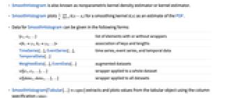
- SmoothHistogram is also known as nonparametric kernel density estimator or kernel estimator.
- SmoothHistogram plots
 for a smoothing kernel
  as an estimate of the PDF.
 - Data for SmoothHistogram can be given in the following forms:
-
{e1,e2,…}list of elements with or without wrappers <|k1y1,k2y2,…|>association of keys and lengths TimeSeries[…],EventSeries[…],TemporalData[…]time series, event series, and temporal data WeightedData[…],EventData[…]augmented datasets w[{e1,e2,…},…]wrapper applied to a whole dataset w[{data1,data1,…},…]wrapper applied to all datasets - The estimator specification espec can be of the form bw or {bw,kernel}.
- The specifications for bandwidth bw and kernel are the same as for SmoothKernelDistribution.
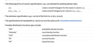
- Possible distribution functions dfun include:
-
"PDF"probability density function "Intensity"count density function "CDF"cumulative distribution function "SF"survival function "HF"hazard function "CHF"cumulative hazard function - The form w[data] provides a wrapper w to be applied to the resulting graphics primitives.
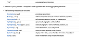
- The following wrappers can be used:
-
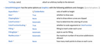
Annotation[e,label]provide an annotation Button[e,action]define an action to execute when the element is clicked EventHandler[e,…]define a general event handler for the element Highlighted[e,effect]dynamically highlight e with an effect Highlighted[e,Placed[effect,pos]]statically highlight e with an effect at position pos Hyperlink[e,uri]make the element act as a hyperlink PopupWindow[e,cont]attach a popup window to the element StatusArea[e,label]display in the status area when the element is moused over Style[e,opts]show the element using the specified styles Tooltip[e,label]attach an arbitrary tooltip to the element - SmoothHistogram has the same options as Graphics with the following additions and changes: [List of all options]
-
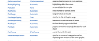
AspectRatio 1/GoldenRatioratio of width to height Axes Truewhether to draw axes ClippingStyle Nonewhat to draw where curves are clipped ColorFunction Automatichow to determine the coloring of curves ColorFunctionScaling Truewhether to scale arguments to ColorFunction Filling Nonefilling to insert under each curve FillingStyle Automaticstyle to use for filling MaxRecursion Automaticthe maximum number of recursive subdivisions allowed Mesh Nonehow many mesh points to draw on each curve MeshFunctions {#1&}how to determine the placement of mesh points MeshShading Nonehow to shade regions between mesh points MeshStyle Automaticthe style for mesh points MethodAutomaticmethods to use PerformanceGoal $PerformanceGoalaspects of performance to try to optimize PlotHighlightingAutomatichighlighting effect for curves PlotPoints Automaticinitial number of sample points PlotRange Automaticrange of values to include PlotRangeClippingTruewhether to clip at the plot range PlotStyle Automaticgraphics directives to specify the style for each object PlotTheme $PlotThemeoverall theme for the plot RegionFunction(True&)how to determine whether a point should be included ScalingFunctionsNonehow to scale individual coordinates WorkingPrecisionMachinePrecisionthe precision used in internal computations for symbolic distributions - Possible settings for PlotLayout that show single curves in multiple plot panels include:
-
"Column"use separate curves in a column of panels "Row"use separate curves in a row of panels {"Column",k},{"Row",k}use k columns or rows {"Column",UpTo[k]},{"Row",UpTo[k]}use at most k columns or rows - The arguments supplied to RegionFunction, MeshFunctions, and ColorFunction are x and f, where f can be the PDF, CDF, etc. of the distribution.
- Possible highlighting effects for Highlighted and PlotHighlighting include:
-
 stylehighlight the indicated curve
 "Ball"highlight and label the indicated point in a curve
 "Dropline"highlight and label the indicated point in a curve with droplines to the axes
 "XSlice"highlight and label all points along a vertical slice
 "YSlice"highlight and labels all points along a horizontal slice
 Placed[effect,pos]statically highlight the given position pos
- Highlight position specifications pos include:
-
x,{x} effect at {x,y} with y chosen automatically {x,y}effect at {x,y} {pos1,pos2,…}multiple positions posi - With ScalingFunctions->{sx,sy}, the
 coordinate is scaled using sx and the
  coordinate is scaled using sy.
 -
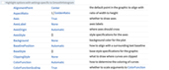
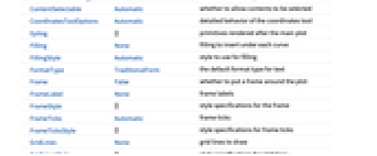
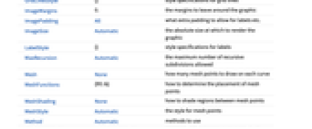
AlignmentPointCenterthe default point in the graphic to align with AspectRatio1/GoldenRatioratio of width to height AxesTruewhether to draw axes AxesLabelNoneaxes labels AxesOriginAutomaticwhere axes should cross AxesStyle{}style specifications for the axes BackgroundNonebackground color for the plot BaselinePositionAutomatichow to align with a surrounding text baseline BaseStyle{}base style specifications for the graphic ClippingStyleNonewhat to draw where curves are clipped ColorFunctionAutomatichow to determine the coloring of curves ColorFunctionScalingTruewhether to scale arguments to ColorFunction ContentSelectableAutomaticwhether to allow contents to be selected CoordinatesToolOptionsAutomaticdetailed behavior of the coordinates tool Epilog{}primitives rendered after the main plot FillingNonefilling to insert under each curve FillingStyleAutomaticstyle to use for filling FormatTypeTraditionalFormthe default format type for text FrameFalsewhether to put a frame around the plot FrameLabelNoneframe labels FrameStyle{}style specifications for the frame FrameTicksAutomaticframe ticks FrameTicksStyle{}style specifications for frame ticks GridLinesNonegrid lines to draw GridLinesStyle{}style specifications for grid lines ImageMargins0.the margins to leave around the graphic ImagePaddingAllwhat extra padding to allow for labels etc. ImageSizeAutomaticthe absolute size at which to render the graphic LabelStyle{}style specifications for labels MaxRecursionAutomaticthe maximum number of recursive subdivisions allowed MeshNonehow many mesh points to draw on each curve MeshFunctions{#1&}how to determine the placement of mesh points MeshShadingNonehow to shade regions between mesh points MeshStyleAutomaticthe style for mesh points MethodAutomaticmethods to use PerformanceGoal$PerformanceGoalaspects of performance to try to optimize PlotHighlightingAutomatichighlighting effect for curves PlotLabelNonean overall label for the plot PlotPointsAutomaticinitial number of sample points PlotRangeAutomaticrange of values to include PlotRangeClippingTruewhether to clip at the plot range PlotRangePaddingAutomatichow much to pad the range of values PlotRegionAutomaticthe final display region to be filled PlotStyleAutomaticgraphics directives to specify the style for each object PlotTheme$PlotThemeoverall theme for the plot PreserveImageOptionsAutomaticwhether to preserve image options when displaying new versions of the same graphic Prolog{}primitives rendered before the main plot RegionFunction(True&)how to determine whether a point should be included RotateLabelTruewhether to rotate y labels on the frame ScalingFunctionsNonehow to scale individual coordinates TicksAutomaticaxes ticks TicksStyle{}style specifications for axes ticks WorkingPrecisionMachinePrecisionthe precision used in internal computations for symbolic distributions
List of all options
Examples
open allclose allBasic Examples (3)
Plot the probability density function of the data:
Cumulative distribution function:
Scope (29)
Data (11)
Plot different distribution functions:
PlotRange is selected automatically:
Use PlotRange to focus on areas of interest:
Non-real data points are ignored:
Specify the number of times to refine the curve:
Override the default tooltips:
Use any object in the tooltip:
Use PopupWindow to provide additional drilldown information:
Numeric values in an association are used as the y coordinates:
Numeric keys and values in an association are used as the x and y coordinates:
The weights in WeightedData are ignored:
Bandwidth and Kernel (9)
Automatically select the bandwidth to use:
More data yields better approximations to the underlying distribution:
Explicitly specify the bandwidth:
Larger bandwidths yield smoother estimates:
Specify bandwidths in units of standard deviation:
Use bandwidths of  and
and  of the standard deviation:
Allow bandwidth to vary adaptively with local density:
Vary the local sensitivity from  (none) to
  (full):
Vary the initial bandwidth for an adaptive estimate:
Specify an initial bandwidth of  and
and  respectively:
Use any of several automatic bandwidth selection methods:
Silverman's method is used by default for bandwidth selection:
Specify any one of several kernel functions:
Define the kernel function as a pure function:
Presentation (9)
Multiple datasets are automatically colored to be distinct:
Provide explicit styling to different sets:
Use rows and columns of individual plots to show multiple sets:
Use the default tooltip for the data:
Provide an interactive tooltip for the data:
Style the curve segments between mesh points:
Options (79)
AspectRatio (4)
By default, SmoothHistogram uses a fixed height to width ratio for the plot:
Make the height the same as the width with AspectRatio1:
AspectRatioAutomatic determines the ratio from the plot ranges:
AspectRatioFull adjusts the height and width to tightly fit inside other constructs:
Axes (4)
Use AxesFalse to turn off axes:
Use AxesOrigin to specify where the axes intersect:
Turn each axis on individually:
AxesLabel (4)
No axes labels are drawn by default:
 axis:
axis:AxesOrigin (2)
The position of the axes is determined automatically:
Specify an explicit origin for the axes:
AxesStyle (4)
Change the style for the axes:
Specify the style of each axis:
Use different styles for the ticks and the axes:
Use different styles for the labels and the axes:
ClippingStyle (4)
Omit clipped regions of the plot:
Show the clipped regions like the rest of the curve:
Show the clipped regions with red lines:
Show the clipped regions as red and thick:
ColorFunction (5)
Color by scaled  and
and  coordinates:
Color with a named color scheme:
Fill with the color used for the curve:
ColorFunction has higher priority than PlotStyle for coloring the curve:
Use Automatic in MeshShading to use ColorFunction:
ColorFunctionScaling (2)
Color the line based on scaled  value:
Color the line based on unscaled  value:
Filling (6)
Use symbolic or explicit values:
By default, overlapping fills combine using opacity:
Fill between curve 1 and the  axis:
axis:
Fill between datasets using a particular style:
Use different styles above and below the filling level:
FillingStyle (4)
Fill with red when the first curve is below the second, and blue when the second is below the first:
Use a variable filling style obtained from a ColorFunction:
ImageSize (7)
Use named sizes such as Tiny, Small, Medium and Large:
Specify the width of the plot:
Specify the height of the plot:
Allow the width and height to be up to a certain size:
Specify the width and height for a graphic, padding with space if necessary:
Setting AspectRatioFull will fill the available space:
Use maximum sizes for the width and height:
Use ImageSizeFull to fill the available space in an object:
Specify the image size as a fraction of the available space:
MaxRecursion (2)
Each level of MaxRecursion will subdivide the initial mesh into a finer mesh:
Mesh (3)
Use 20 mesh levels evenly spaced in the  direction:
Use an explicit list of values for the mesh in the  direction:
Specify and mesh levels and styles in the  direction:
MeshFunctions (2)
Use a mesh evenly spaced in the  and
and  directions:
Show five mesh levels in the  direction (red) and 10 in the
  direction (blue):
MeshShading (6)
Alternate red and blue segments of equal width in the  direction:
Use None to remove segments:
MeshShading can be used with PlotStyle:
MeshShading has higher priority than PlotStyle for styling the curve:
Use PlotStyle for some segments by setting MeshShading to Automatic:
MeshShading can be used with ColorFunction:
MeshStyle (4)
Color the mesh the same color as the plot:
Use a red mesh in the  direction:
Use a red mesh in the  direction and a blue mesh in the
  direction:
Use big, red mesh points in the  direction:
PerformanceGoal (2)
Generate a higher-quality plot:
Emphasize performance, possibly at the cost of quality:
PlotLayout (3)
Place each histogram in a separate panel using shared axes:
Use a row instead of a column:
PlotPoints (1)
Use more initial points to get a smoother curve:
PlotRange (2)
PlotRange is automatically calculated:
SmoothHistogram automatically chooses the plotting domain:
Plot over the middle 90% of the data:
PlotStyle (6)
Use different style directives:
By default, different styles are chosen for multiple curves:
Explicitly specify the style for different curves:
PlotStyle can be combined with ColorFunction:
PlotStyle can be combined with MeshShading:
MeshStyle by default uses the same style as PlotStyle:
PlotTheme (2)
Use a theme with simple ticks and grid lines in a high contrast color scheme:
Applications (4)
The velocities in km/sec of 82 galaxies from six well-separated conic sections of an unfilled survey of the Corona Borealis region. Multimodality in such surveys is evidence for voids and superclusters in the far universe:
Multiple modes are readily detected for a variety of bandwidths:
Observe the density over many possible bandwidths and choose one that captures important features of the data while smoothing out noise. For presentation, it is best to choose a bandwidth that slightly undersmooths the data:
Choosing 6.0 seems to capture the important features of the snowfall data:
Visually compare data to a parametric model of its density:
Smooth histogram for the slice distribution of a random process:
Smooth histogram for several slices of a process:
Properties & Relations (5)
SmoothHistogram effectively plots the distribution function of SmoothKernelDistribution:
Use Histogram to plot the data in discrete bins:
Use SmoothDensityHistogram and SmoothHistogram3D for bivariate data:
Additional points will result in a better approximation of the underlying distribution:
As the bandwidth approaches infinity, the estimate approaches the shape of the kernel:
Possible Issues (1)
Using SmoothHistogram with multivariate data will plot multiple curves:
Neat Examples (1)
A visual explanation of kernel density estimation:
The estimate results from mixing the kernel functions placed at each data point:
Text
Wolfram Research (2010), SmoothHistogram, Wolfram Language function, https://reference.wolfram.com/language/ref/SmoothHistogram.html (updated 2023).
CMS
Wolfram Language. 2010. "SmoothHistogram." Wolfram Language & System Documentation Center. Wolfram Research. Last Modified 2023. https://reference.wolfram.com/language/ref/SmoothHistogram.html.
APA
Wolfram Language. (2010). SmoothHistogram. Wolfram Language & System Documentation Center. Retrieved from https://reference.wolfram.com/language/ref/SmoothHistogram.html