Details and Options

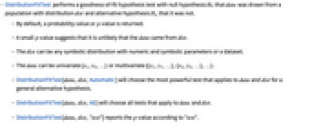
• DistributionFitTest performs a goodness-of-fit hypothesis test with null hypothesis that data was drawn from a population with distribution dist and alternative hypothesis that it was not.
• By default, a probability value or -value is returned.
• A small -value suggests that it is unlikely that the data came from dist.
• The dist can be any symbolic distribution with numeric and symbolic parameters or a dataset.
• The data can be univariate {x₁,x₂,…} or multivariate {{x₁,y₁,…},{x₂,y₂,…},…}.
• DistributionFitTest[data,dist,Automatic] will choose the most powerful test that applies to data and dist for a general alternative hypothesis.
• DistributionFitTest[data,dist,All] will choose all tests that apply to data and dist.
• DistributionFitTest[data,dist,"test"] reports the -value according to "test".
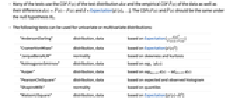
• Many of the tests use the CDF of the test distribution dist and the empirical CDF of the data as well as their difference and =Expectation[d(x),…]. The CDFs and should be the same under the null hypothesis .
• The following tests can be used for univariate or multivariate distributions:
• "AndersonDarling"distribution, databased on Expectation[] "CramerVonMises"distribution, databased on Expectation[d(x)²] "JarqueBeraALM"normalitybased on skewness and kurtosis "KolmogorovSmirnov"distribution, databased on "Kuiper"distribution, databased on "PearsonChiSquare"distribution, databased on expected and observed histogram "ShapiroWilk"normalitybased on quantiles "WatsonUSquare"distribution, databased on Expectation[]
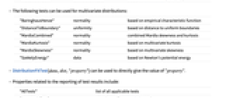
• The following tests can be used for multivariate distributions:
• "BaringhausHenze"normalitybased on empirical characteristic function "DistanceToBoundary"uniformitybased on distance to uniform boundaries "MardiaCombined"normalitycombined Mardia skewness and kurtosis "MardiaKurtosis"normalitybased on multivariate kurtosis "MardiaSkewness"normalitybased on multivariate skewness "SzekelyEnergy"databased on Newton's potential energy
• DistributionFitTest[data,dist,"property"] can be used to directly give the value of "property".
• Properties related to the reporting of test results include:
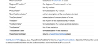
• "AllTests"list of all applicable tests "AutomaticTest"test chosen if Automatic is used "DegreesOfFreedom"the degrees of freedom used in a test "PValue"list of -values "PValueTable"formatted table of -values "ShortTestConclusion"a short description of the conclusion of a test "TestConclusion"a description of the conclusion of a test "TestData"list of pairs of test statistics and -values "TestDataTable"formatted table of -values and test statistics "TestStatistic"list of test statistics "TestStatisticTable"formatted table of test statistics "HypothesisTestData"returns a HypothesisTestData object
• DistributionFitTest[data,dist,"HypothesisTestData"] returns a HypothesisTestData object htd that can be used to extract additional test results and properties using the form htd["property"].
• Properties related to the data distribution include:
• "FittedDistribution"fitted distribution of data "FittedDistributionParameters"distribution parameters of data
• The following options can be given:
• Method Automaticthe method to use for computing -values SignificanceLevel 0.05cutoff for diagnostics and reporting
• For a test for goodness of fit, a cutoff is chosen such that is rejected only if . The value of used for the "TestConclusion" and "ShortTestConclusion" properties is controlled by the SignificanceLevel option. By default, is set to 0.05.
• With the setting Method->"MonteCarlo", datasets of the same length as the input s_i are generated under using the fitted distribution. The EmpiricalDistribution from DistributionFitTest[s_i,dist,{"TestStatistic",test}] is then used to estimate the -value.

Examples

Basic Examples  (3)

Test some data for normality:

Create a HypothesisTestData object for further property extraction:

The full test table:

Compare the histogram of the data to the PDF of the test distribution:

Test the fit of a set of data to a particular distribution:

Extract the Anderson–Darling test table:

Verify the test results with ProbabilityPlot:

Test data for goodness of fit to a multivariate distribution:

Plot the marginal PDFs of the test distribution against the data to confirm the test results:

Scope  (22)

Testing  (16)

Test some data for normality:

The -values for the normally distributed data are typically large:

The -values for data that is not normally distributed are typically small:

Set the third argument to Automatic to apply a generally powerful and appropriate test:

The property "AutomaticTest" can be used to determine which test was chosen:

Test whether data fits a particular distribution:

There is insufficient evidence to reject a good fit to a WeibullDistribution[1,2]:

Test for goodness of fit to a derived distribution:

The -value is large for the mixture data compared to data not drawn from the mixture:

Test for goodness of fit for quantity data:

Check for normality:

Check goodness-of-fit for a specific distribution:

Test for goodness of fit to a formula-based distribution:

Unspecified parameters will be estimated from the data:

The -value is dependent on which parameters were estimated:

Test some data for multivariate normality:

The -values for normally distributed data are typically large compared to non-normal data:

Test some data for goodness of fit to a particular multivariate distribution:

Test a MultinormalDistribution and multivariate UniformDistribution, respectively:

Compare the distributions of two datasets:

The sample sizes need not be equal:

Compare the distributions of two multivariate datasets:

The -values for equally distributed data are large compared to unequally distributed data:

Perform a particular goodness-of-fit test:

Any number of tests can be performed simultaneously:

Perform all tests, appropriate to the data and distribution, simultaneously:

Use the property "AllTests" to identify which tests were used:

Create a HypothesisTestData object for repeated property extraction:

The properties available for extraction:

Extract some properties from a HypothesisTestData object:

The -value and test statistic from a Cramér–von Mises test:

Extract any number of properties simultaneously:

The results from the Anderson–Darling -value and test statistic:

Data Properties  (2)

Obtain the fitted distribution when parameters have been unspecified:

Extract the parameters from the fitted distribution:

Plot the PDF of the fitted distribution against the data:

Confirm the fit with a goodness-of-fit test:

The test distribution is returned when the parameters have been specified:

Visually compare the data to the fitted distribution:

Reporting  (4)

Tabulate the results from a selection of tests:

A full table of all appropriate test results:

A table of selected test results:

Retrieve the entries from a test table for customized reporting:

The -values are above 0.05, so there is not enough evidence to reject normality at that level:

Tabulate -values for a test or group of tests:

The -value from the table:

A table of -values from all appropriate tests:

A table of -values from a subset of tests:

Report the test statistic from a test or group of tests:

The test statistic from the table:

A table of test statistics from all appropriate tests:

Options  (6)

Method  (4)

Use Monte Carlo-based methods, or choose the fastest method automatically:

Set the number of samples to use for Monte Carlo-based methods:

The Monte Carlo estimate converges to the true -value with increasing samples:

Set the random seed used in Monte Carlo-based methods:

The seed affects the state of the generator and has some effect on the resulting -value:

Monte Carlo simulations generate many test statistics under :

The estimated distribution of the test statistics under :

The empirical estimate of the -value agrees with the Monte Carlo estimate:

SignificanceLevel  (2)

By default, a significance level of 0.05 is used:

Set the significance level to 0.001:

The significance level is also used for "ShortTestConclusion":

Applications  (12)

Analyze whether a dataset is drawn from a normal distribution:

Perform a series of goodness-of-fit tests:

Visually compare the empirical and theoretical CDFs in a QuantilePlot:

Visually compare the empirical CDF to that of the test distribution:

Determine whether snowfall accumulations in Buffalo are normally distributed:

Use the Jarque–Bera ALM test and Shapiro–Wilk test to assess normality:

The SmoothHistogram agrees with the test results:

The QuantilePlot suggests a reasonably good fit:

Use a goodness-of-fit test to verify the fit suggested by visualization such as a histogram:

The Kolmogorov–Smirnov test agrees with the good fit suggested in the histogram:

Test whether the absolute magnitudes of the 100 brightest stars are normally distributed:

The value of the statistic and p-value for the automatic test:

Visually check the result:

Test whether multivariate data is uniformly distributed over a box:

Use the distance-to-boundary test:

Use Szekely's energy test to compare two multivariate datasets:

The distributions for measures of counterfeit and genuine notes are significantly different:

Visually compare the marginal distributions to determine the origin of the discrepancy:

Test whether data is uniformly distributed on a unit circle:

Kuiper's test and the Watson test are useful for testing uniformity on a circle:

The first dataset is randomly distributed, the second is clustered:

Determine if a model is appropriate for day-to-day point changes in the S&P 500 index:

The histogram suggests a heavy-tailed, symmetric distribution:

Try a LaplaceDistribution:

For very large datasets, small deviations from the test distribution are readily detected:

Test the residuals from a LinearModelFit for normality:

The Shapiro–Wilk test suggests that the residuals are not normally distributed:

The QuantilePlot suggests large deviations in the left tail of the distribution:

Simulate the distribution of a test statistic to obtain a Monte Carlo -value:

Visualize the distribution of the test statistic using SmoothHistogram:

Obtain the Monte Carlo -value from an Anderson–Darling test:

Compare with the -value returned by DistributionFitTest:

Obtain an estimate of the power for a hypothesis test:

Visualize the approximate power curve:

Estimate the power of the Shapiro–Wilk test when the underlying distribution is a StudentTDistribution[2], the test size is 0.05, and the sample size is 35:

Smoothing a dataset using kernel density estimation can remove noise while preserving the structure of the underlying distribution of the data. Here two datasets are created from the same distribution:

The unsmoothed data provides a noisy estimate of the underlying distributions:

Noise would lead to committing a type I error:

Smoothing reduces the noise and results in a correct conclusion at the 5% level:

Properties & Relations  (16)

By default, univariate data is compared to a NormalDistribution:

The parameters of the distribution are estimated from the data:

Multivariate data is compared to a MultinormalDistribution by default:

Unspecified parameters of the distribution are estimated from the data:

Maximum likelihood estimates are used for unspecified parameters of the test distribution:

The -value suggests the expected proportion of false positives (type I errors):

Setting the size of a test to 0.05 results in an erroneous rejection of about 5% of the time:

Type II errors arise when is not rejected, given it is false:

Increasing the size of the test lowers the type II error rate:

The -value for a valid test has a UniformDistribution[{0,1}] under :

Verify the uniformity using the Kolmogorov–Smirnov test:

The power of each test is the probability of rejecting when it is false:

Under these conditions, the Pearson test has the lowest power:

The power of each test decreases with sample size:

Some tests perform better than others with small sample sizes:

Some tests are more powerful than others for detecting differences in location:

The power of the tests:

Some tests are more powerful than others for detecting differences in scale:

The power of the tests:

The Pearson test requires large sample sizes to have high power:

The power of the tests:

Some tests perform better than others when testing normality:

The Jarque–Bera ALM and Shapiro–Wilk tests are the most powerful for small samples:

Tests designed for the composite hypothesis of normality ignore specified parameters:

Different tests examine different properties of the distribution. Conclusions based on a particular test may not always agree with those based on another test:

The green region represents a correct conclusion by both tests. Points fall in the red region when a type II error is committed by both tests. The gray region shows where the tests disagree:

Estimating parameters prior to testing affects the distribution of the test statistic:

The distribution of the test statistics and resulting -values under :

Failing to account for the estimation leads to an overestimate of -values:

The distribution fit test works with the values only when the input is a TimeSeries:

Possible Issues  (5)

Some tests require that the parameters be prespecified and not estimated for valid -values:

It is usually possible to use Monte Carlo methods to arrive at a valid -value:

For many distributions, corrections are applied when parameters are estimated:

The Jarque–Bera ALM test must have sample sizes of at least 10 for valid -values:

Use Monte Carlo methods to arrive at a valid -value:

The Kolmogorov–Smirnov test and Kuiper's test expect no ties in the data:

The Jarque–Bera ALM test and Shapiro–Wilk test are only valid for testing normality:

Careful interpretation is required when some tests are used for discrete distributions:

The Pearson test applies directly for discrete distributions:

Neat Examples  (1)

The distributions of some test statistics: